Methodology

from a BASH script to a binary-search catchment engine

From a script to a model

Early attempts at the modelling process involved scripts written in BASH. BASH (Bourne-Again SHell) is a Unix shell and scripting language. Useful for orchestrating GIS commands; not ideal for stateful, complex domain logic. Incorporating multiple factors — different crops and animals, fallow rotation, fallow grazing — into an integrated working model made it evident that a script was not going to be ideal. The complexity of the animal and crop modelling in particular made using scripts very awkward. While the scripting approach worked well for a proof of concept, a full implementation would include a large number of hard-coded variables and complicated hard-to-debug code.

The scripting approach also had poor reporting capabilities and could offer little guidance to the user as the analysis was carried out. Consultation with developers of other modelling software led to the decision to create an application in C++ using Qt libraries to create a user-friendly GUI. The original Landuse Analyst was a desktop application; later it was ported to a QGIS plugin in C++, then in 2026 to Python, then to this web app. This research analyses multiple sites, so the software was designed to be flexible enough to use without modification on any site, by allowing all of the influencing factors to be entered as input variables.

What began as a small script has grown into a flexible, user-friendly application that can be used not only for the research presented in the original thesis, but by any archaeologist studying any time period, for any type of crop or animal, in any area of the world. Landuse Analyst is released as Free, Open Source Software (FOSS) under the GPL because it incorporates code from other applications that are also licensed this way — notably GRASS GIS.

The five-step model

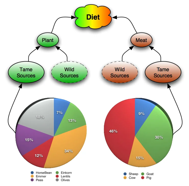
Landuse Analyst calculates the amount of agricultural land a settlement needs in five steps:

1. Break the diet down into specific crops and animals being used for nourishment. Each individual crop and animal is expressed as a percentage of the people's diet, estimated from archaeological evidence such as faunal and palaeobotanical remains.
2. Calculate calorie targets for the crops and animals identified above. Total daily calorific requirement × population × dietary proportions.
3. Calculate production targets that fulfil the calorie targets. Production is in kilograms, and takes into account factors such as calories per kg of produce, and what percentage of an animal's weight is usable as food.
4. Calculate land-area targets needed to satisfy the production targets. Each crop and animal is allocated a specific area target.
5. Carry out a spatial analysis of the land surrounding the settlement to find land suitable for each crop and animal that satisfies the area targets.

This site focuses on step five — the spatial catchment analysis — because it's the GIS-heavy part that benefits most from a live interactive tool. The diet → calorie → production → area pipeline (steps 1–4) is still implemented in the engine and visible in the Explorer's scenario settings, but it involves a lot of input fields and is best done in the desktop application.

Finding the land: the catchment search

Once area targets are known, the model needs to find the land surrounding the settlement that is suitable for the right kinds of agriculture and which, in total, satisfies those targets — in closest proximity to the settlement. A conditional loop defines the outer extent of the catchment area and calculates the area of suitable land contained within it.

Earlier versions of Landuse Analyst started at the closest point to the site that could potentially solve the problem The closest point — or minimum radius — is a perfect circle equal in area to the target. Anything inside that radius is trivially too small; anything just outside has potential. and then moved steadily outwards until the area target was found. The amount to move outward in each step was provided by the user. This worked but was extremely slow: with even 3,500 loops, at 45 seconds each, the computation time was nearly 44 hours. Multiply by the number of crops and animals and the run time was measured in days or weeks.

The binary-search optimisation

To increase the efficiency, a modified binary search is now used. Instead of a step amount, a precision percentage is used. The area of land deemed by the engine as equalling the current area target gets relaxed into a target range:

If a value of $p=5\%$ is entered and the area target is $A_{\text{target}}=100$ hectares, the engine accepts the range $[97.5,102.5]$ hectares as the target area.

The loop uses three terms — CurrentMidValue, FirstValue, and LastValue. At the beginning, FirstValue = 0 and LastValue = 40,000, the full extent of the cost surface in seconds of walking time. The loop:

1. Set the analysis boundary: $\text{CurrentMidValue}=\frac{\text{FirstValue}+\text{LastValue}}{2}$
2. Calculate the area of suitable land found within the boundary defined by CurrentMidValue.
3. If the contained area falls within the target range, write the results and exit.
4. If the contained area is more than the maximum, set LastValue = CurrentMidValue and return to step 1.
5. If the contained area is less than the minimum, set FirstValue = CurrentMidValue and return to step 1.

By construction, the maximum number of iterations is 17 — at which point the search resolution is smaller than the precision and the result is the closest match achievable. A typical run on a modern laptop is now ~150 ms for the windowed Shuna scenario; the original step-amount approach would have taken hours for the same problem.

Watch the search converge

Below is a real iteration trace from the Shuna cost surface, binary-searching for a deliberately-chosen demonstration target of $8,000$ hectares with ±0.5% precision — picked because it sits on a steep part of the threshold-vs-area curve, where the search has to swing genuinely back and forth (too much · too little · too much · too little) before homing in. The bracket starts at $[0,40,000]$ seconds — covering the engine's full search range — and the X-axis is auto-zoomed to $24,000\text{s}$ so the bracket-narrowing dance sits inside the chart rather than bunching at the left edge. Eleven iterations total, seven sign flips between over and under, converging at mid $\approx 5,840$ seconds (achieved 7,989 Ha, delta < 11 Ha).

Hit Play and watch the runner (down in the status panel) sprint along with the search — frantic on the early big-delta iterations, more measured as the bracket tightens, triumphant when the threshold finally lands inside the FINISH window. Flip Crayon Mode for hand-drawn annotations.

The cost surface

The "boundary" referred to above is a cost-distance threshold, not a physical radius. Two cells equidistant from the settlement in metres may be very different in walking time if one is up a steep slope and the other is on flat ground. The cost surface is built using Tobler's hiking function Tobler, W. (1993). Three Presentations on Geographical Analysis and Modeling. NCGIA Technical Report 93-1. , which weights each edge in an 8-connected DEM grid by signed slope:

with default parameters $V_{\text{peak}}=6.0\text{ km/h}$, slope-penalty $K=3.5$, and a slight downhill bias of $b=0.05$. The asymmetry means walking gently downhill is faster than walking the same gradient uphill. Dijkstra's algorithm then propagates accumulated cost from the settlement seed through the directed cost graph; cells beyond ~11 h of walking are masked unreachable.

Dynamic 3D Terrain Tiles

To render the topography in 3D directly in the browser, the web app hosts a custom Web Mercator tile server. The server dynamically reprojects the scenario's underlying DEM elevation model and encodes the heights into Mapbox Terrain-RGB pixels:

MapLibre GL JS decodes these pixels on the fly to render realistic terrain relief, allowing vertical exaggeration adjustments from 1.0x to 5.0x.

Explore the function

The Tobler velocity curve is asymmetric and decays sharply for steep terrain. Drag the sliders to see how each parameter shapes it — the grey dashed line shows the canonical Tobler 1993 form for comparison, and the orange dotted lines are reference walking speeds from Bohannon (1997). Bohannon, R. W. (1997). "Comfortable and maximum walking speed of adults aged 20–79 years: reference values and determinants." Age and Ageing, 26(1), 15–19. Values are converted from cm/s in the original source. The pedagogical anchor: Tobler's 6 km/h peak sits between women's comfortable and men's maximum walking paces — exactly where a "normal walking" peak should sit.

Why this matters for the catchment: a settlement whose surrounding terrain has a lot of gentle downhill (a hilltop site overlooking a valley, say) will have a much larger walking-time catchment than one in the middle of a flat plain — even though both look identical on a Euclidean-distance map. Conversely, an uphill approach from the valley floor (Shuna is a Jordan-Valley-floor site overlooked by sharp terraces) collapses the catchment on that side of the settlement.

Land suitability

A cost surface alone is not enough — not every reachable cell is agriculturally useful. Land-suitability rasters constrain the catchment to cells that meet ecological criteria for each crop/animal. The engine is designed to compose any combination of factors — slope, soil type, elevation band, rainfall, salinity, crop-rotation patterns, microclimate — by intersecting per-factor masks before the catchment search runs. "The simple approach taken in this thesis was to use only one classification factor (slope), but Landuse Analyst has been specifically designed to use any combination of factors." — Jorgenson (2022), § 7.2 p. 366. The catchment for any given crop is the intersection of "reachable within threshold T" and "suitable for crop X under all chosen factors."

Friction Barriers & Vector Routing

To simulate real-world travel obstacles (like rivers and lakes), the web app integrates vector drawing tools. When a user draws a barrier, it is saved as GeoJSON and rasterized onto the analysis grid:

• Line features (rivers): Rasterized with a custom crossing penalty (expressed in minutes). The penalty is converted into seconds per meter of friction and added to the Tobler edge weights during Dijkstra routing.
• Polygon features (lakes): Rasterized with a near-infinite friction multiplier ($10^7$), rendering the cells completely impassable.

The engine's pathfinder automatically computes anisotropic walking routes around these obstacles, shifting agricultural allocations to more reachable sectors.

The thesis case study at Shuna used slope alone — separate binary masks at ≤ 9° for cropland and ≤ 15° for grazing land, after Joolen (2003) — and the preloaded scenario on this site additionally uses an elevation-band mask (Jordan-Valley floor) as the baseline suitability layer. Research scenarios can stack richer factor layers (soil maps, vegetation, rainfall) on top.

Scope of the case study

The thesis case study was deliberately a single-site, single-day, fixed-population snapshot — settlement as a point, walk to the fields and back in one day. The engine itself supports a broader research surface that the thesis case study did not exercise: multi-year fallow rotations with three-level fallow-grazing access priority, surplus tracking with inter-site trade modelling, mutual-aid scenarios between neighbouring settlements, drought / crop-failure responses, and emergency consumption of breeding stock. These workflows are described in Jorgenson (2022), § 7.2 "Methodological Development and Future Work", pp. 364–367. Some are already accessible through the engine API; surfacing them in this web UI is ongoing work. The regional climax of the thesis — Thiessen polygons, XTent modelling, walking-time path networks, and regional-scale catchment overlap analysis applied to 126 EB I sites — is Chapter 6 of the thesis. The first piece of it, Thiessen tessellation, is now live on the regional explorer; XTent and the path-network analysis follow next.

Scaling to a region

Chapter 6 of the thesis steps out from the single-settlement case study to look at Shuna in conjunction with 125 other Early Bronze I sites across the southern Levant. Three territory-allocation methods are compared: Thiessen polygons (the simplest, equal-weight tessellation), Renfrew and Level's XTent model (which weights each site's influence by its size), and Landuse Analyst catchments themselves (which respond to the actual terrain). Jorgenson (2022), § 6.3 "Thiessen Polygons and XTent Modelling", pp. 333–336. The regional explorer on this site now ships Thiessen polygons, Renfrew & Level's XTent model, and walking-time path networks computed with Tobler hiking costs over a digital-elevation model (§ 6.4) Jorgenson (2022), § 6.4 "Path Networks", pp. 337–342. The thesis ran this analysis on 627 EB I sites using GRASS r.walk + r.drain across multiple machines for several days; this site does the five EB I stubs that fall within the Shuna DEM coverage in under thirty seconds. Routes are computed in both directions per the thesis's anisotropic-Tobler treatment; pairs where climbing and descending costs diverge appear as two parallel paths. Way-point optimisation per § 6.4 p. 339 is applied by default: a multi-origin cost surface is generated and used as a friction map on the per-site routes, so traffic bundles through corridors near other settlements rather than empty wilderness. . Eight named EB I sites near Shuna are seeded as picker options with approximate hectare-size estimates; the southern three (Jericho, Ai, Tell el-Hammam) fall outside the current DEM and so produce territorial polygons but no walking routes. The only Ch 6 piece still to land is the regional catchment-overlap analysis of § 6.5.

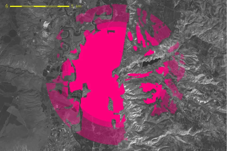
A sample result

The final output of the model is a set of catchment masks, one per crop and one per animal, plus the cost surface that produced them. Below is a sample result from the original thesis run: the blue cells are land identified as agricultural catchment, the green cells as grazing land, computed at a particular population and dietary configuration around Shuna.

Flat-Terrain Diagnostics

On highly uniform, flat terrain (such as the Jordan Valley floor), the Tobler walking velocity collapses to a constant. Over an 8-connected grid, Dijkstra's shortest-path algorithm over uniform costs produces a regular octagon (the shape of the $L_{\infty }$ unit ball).

To prevent users from misinterpreting these regular shapes as software bugs, the web app computes the elevation range ($\max -\min$) and the percentage of cells eliminated by the slope cap. If the elevation range within the catchment is small (< 5 m) and the slope cap is not binding, the UI displays a diagnostic warning: "Flat Terrain Warning: Catchment geometry may be octagonal due to uniform Dijkstra routing."