Agricultural Catchment Model
The Agricultural Catchment Model is Landuse Analyst’s core spatial solver. It calculates the land area required to sustain a human settlement based on caloric demand, crop productivity, soil fertility, slope penalties, and travel-time constraints.
Given a settlement centroid and demographic parameters, the engine propagates outward across the underlying terrain — constructing Von Thünen land-use rings (intensive arable cultivation, pastoral grazing, and firewood collection) and evaluating whether the site achieves caloric self-sufficiency.
Access: The Catchment Model is open to all visitors at
/model.
When to use it
- Assess settlement viability. Can an Early Bronze Age population of 1,200 inhabitants at Tell esh-Shuna North sustain itself within a 1-hour walking radius?
- Test crop allocation scenarios. How does shifting crop mix from $65%$ cereal / $20%$ pulses to an olive-dominated orchard regime alter the site’s territorial footprint?
- Evaluate terrain slope impedance. How severely do steep slope gradients in the Jordan Valley escarpment limit outward agricultural expansion?
- Compare propagation geometries. Contrast simple radial Euclidean buffers against anisotropic octagonal cell cost surfaces.
Anatomy of the interface
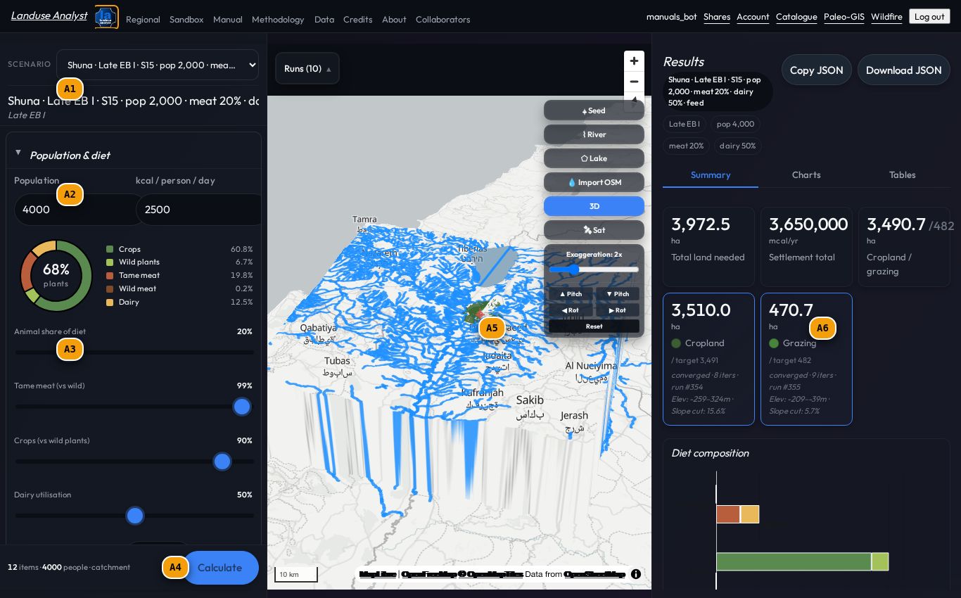
The Catchment Model interface pairs a scrolling Control Sidebar on the left with a full-viewport Map Canvas on the right.
| Tag | Control | What it does |
|---|---|---|
A1 | Site Selection Accordion | Select pre-configured archaeological benchmark sites (e.g. Tell esh-Shuna N., Jericho, Khirbet ez-Zeraqon) or enter custom lat/lon coordinates. |
A2 | Population & Demographics | Set settlement population count ($P$), daily per-capita caloric requirement (default $2,100 \text{ kcal/person/day}$), and demographic distribution. |
A3 | Crop Mix & Yield Allocation | Configure crop proportions (wheat/barley vs pulses vs olives), baseline yields ($\text{kg/ha}$), and biennial fallow practices. |
A4 | Friction & Propagation Settings | Select octagonal grid vs radial propagation, slope penalty function (Minetti equation), and maximum walking time cutoff. |
A5 | Compute Button | Submits the scenario to the spatial engine and renders the resulting catchment rings on the map canvas. |
A6 | Catchment Centroid Marker | Map pin marking the settlement center. Drag to reposition the settlement over new terrain. |
A7 | Results Summary Overlay | HUD panel reporting total arable hectares, caloric self-sufficiency percentage, annual surplus/deficit, and total labor hours. |
Input parameters & calibration levers
Doing it this way allowed me to decouple demographic demand from physical land capability, ensuring that every variable — from caloric density to slope-induced energy expenditure — carries a transparent receipt.
| Tag | Parameter Control | Range / Options | Default | Computational Effect |
|---|---|---|---|---|
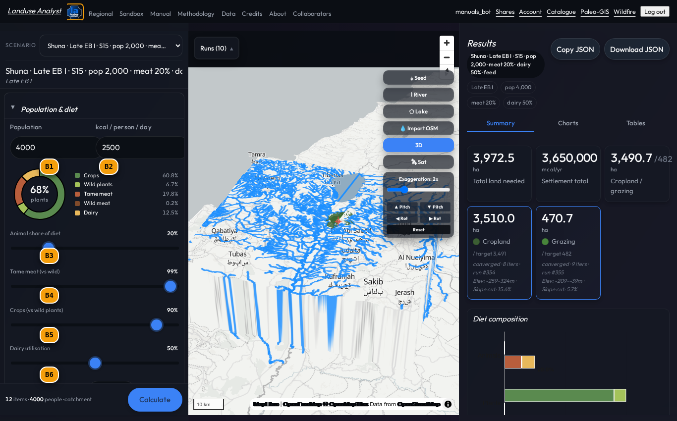
B1 | Settlement Population | 50 – 50,000 persons | 1,200 | Directly scales total annual caloric requirement: $E_{\text{total}} = P \times E_{\text{daily}} \times 365$. |
B2 | Per-Capita Daily Demand | 1,500 – 3,500 kcal/day | 2,100 | Standard caloric intake baseline adjusted for age/gender distribution. |
B3 | Cereal Crop Fraction | 0% – 100% | 65% | Land fraction dedicated to wheat and barley (yield $\approx 1,200 \text{ kg/ha}$; $3,300 \text{ kcal/kg}$). |
B4 | Pulse Crop Fraction | 0% – 100% | 20% | Land fraction dedicated to legumes (lentil, chickpea; yield $\approx 800 \text{ kg/ha}$; $3,400 \text{ kcal/kg}$). |
B5 | Grid Propagation Model | octagonal / radial | octagonal | Octagonal 8-neighbor cost-grid propagation eliminates Manhattan diagonal distortion ($d$ orthogonal, $\sqrt{2}d$ diagonal). |
B6 | Slope Penalty Model | minetti / tobler / flat | minetti | Applies metabolic cost curve vs terrain incline: $C_w(i) = 280.5 i^5 - 58.7 i^4 + 33.2 i^3 + 1.8 i^2 + 7.8 i + 2.5$. |
Walkthrough: Running a Catchment Simulation
Follow these steps to analyze an agricultural site:
1. Select a Benchmark Site
- Expand the Site Selection accordion (
A1). - Pick Tell esh-Shuna N. from the dropdown. The map automatically pans to the Northern Jordan Valley ($32.61^\circ\text{N}, 35.61^\circ\text{E}$).
2. Set Demographics & Crop Requirements
- In Population & Demographics (
A2), set the population slider (B1) to 1,200 persons. - Keep the daily caloric baseline (
B2) at 2,100 kcal/day. - In Crop Mix (
A3), verify the 65% cereal / 20% pulse / 15% olive split with biennial fallow enabled ($\beta = 2.0$).
3. Configure Propagation Geometry
- In Friction & Slope (
A4), ensure Octagonal Propagation (B5) and Minetti Slope Penalty (B6) are selected. - Set the maximum walking radius cutoff to 60 minutes (1-hour walk limit).
4. Execute and Read Results
- Click COMPUTE CATCHMENT (
A5). - Inspect the map canvas (
A6):- Blue Inner Zone: Intensive arable cultivation ring.
- Amber Outer Ring: Pastoral grazing and firewood collection zone.
- Review the Results Summary HUD (
A7):- Total Arable Area: $412.5\text{ ha}$
- Caloric Self-Sufficiency: $108.4%$
- Annual Surplus: $+77.2 \times 10^6\text{ kcal/yr}$
How it works
The question, then, is how to model catchment expansion without falling into the trap of isotropic circular buffers. Real agriculturalists do not walk in perfect circles — they follow paths of least resistance across slope contours and river crossings.
The Catchment Model uses an 8-neighbor octagonal cost-propagation algorithm across a $30\text{ m}$ digital elevation grid.
- Caloric Self-Sufficiency Ratio ($\mathbb{S}$): $$\mathbb{S} = \frac{\sum_{c} \left( A_c \times Y_c \times K_c \right)}{P \times E_{\text{daily}} \times 365} \times 100%$$ Where $A_c$ is cultivated crop area, $Y_c$ is yield ($\text{kg/ha}$), and $K_c$ is caloric density ($\text{kcal/kg}$).
- Fallow Multiplier: A 1:1 biennial fallow regime ($\beta = 2.0$) doubles the required arable footprint, accounting for land resting in alternate years.
Related Manuals
- Barriers & Travel-Time Sandbox — Explore travel friction surfaces and river crossing penalties.
- Methodology & Formulations — Mathematical equations governing caloric yields and octagonal cell propagation.
- Glossary — Definitions for Von Thünen rings, Minetti slope penalties, and fallow ratios.