Barriers & Travel-Time Sandbox
The Barriers & Travel-Time Sandbox is an interactive spatial tool for modelling human movement, travel friction, slope velocity penalties, and barrier permeability across digital elevation models (DEMs).
By integrating Tobler’s Hiking Function with land-cover friction weights and hydrographic barrier penalties, the Sandbox calculates anisotropic travel-time surfaces and renders accessibility isochrone contours around any origin point.
Access: The Barriers Sandbox is open to all visitors at
/sandbox.
When to use it
- Probe landscape accessibility. How far can an individual walk on foot in 60 minutes across the rugged topography surrounding the Dead Sea?
- Test river permeability. See how adding a $5.0\times$ friction penalty along the Jordan River deforms travel-time contours — and how ford crossings restore movement.
- Compare hiking velocity models. Contrast Tobler’s empirical exponential function against Naismith’s Rule, Minetti’s metabolic equation, or Imhof’s slope model.
- Feed the Catchment Model. Generate travel-time cost rasters that feed directly into arable land boundary calculations.
Anatomy of the interface
The Sandbox workspace consists of a scrolling Friction & Parameter Sidebar on the left and an interactive Isochrone Map Viewport on the right.
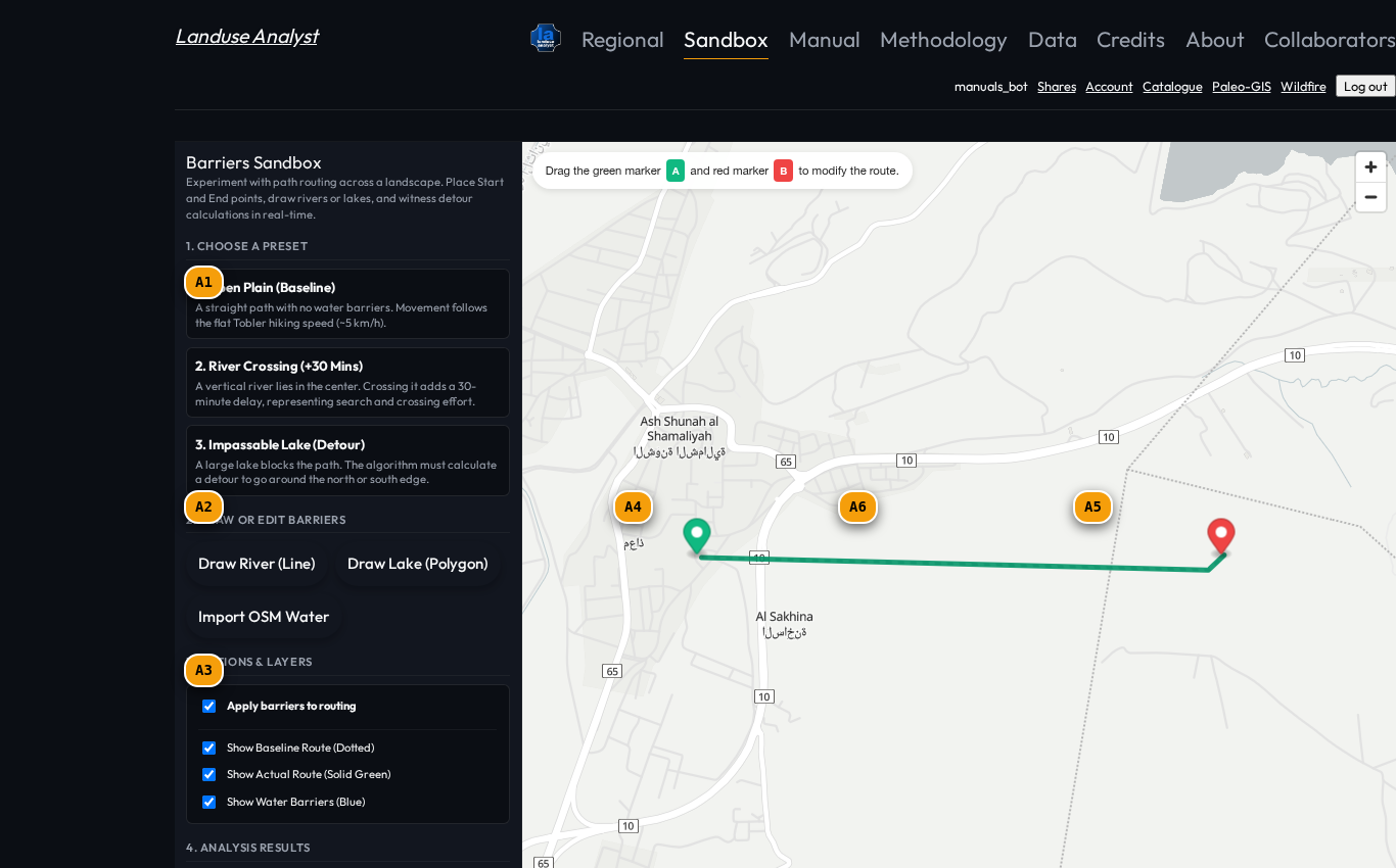
| Tag | Control | What it does |
|---|---|---|
A1 | Hiking Function Selector | Choose walking velocity model: Tobler (1993) (default), Naismith’s Rule, Minetti (1987), or Imhof (1950). |
A2 | Barrier & River Penalties | Configure friction multipliers for major rivers (e.g. Jordan River), wadi gullies, steep escarpments, and permeable ford sites. |
A3 | Isochrone Contour Interval | Set time interval for accessibility contours (e.g. 15 min, 30 min, 60 min) and maximum travel-time cutoff (up to 300 min). |
A4 | Origin Marker | Draggable origin pin on the map. Drag anywhere to recalculate anisotropic travel time from that location. |
A5 | Ford / Pass Identifiers | Green markers highlighting permeable crossing sites (bridges, shallow river fords, mountain passes). |
A6 | Travel-Time Isochrones | Colour-coded accessibility contours showing 15-min (blue), 30-min (amber), and 60-min (red) travel boundaries. |
Walking velocity & slope formulation
The Sandbox defaults to Tobler’s Hiking Function (1993), an empirical exponential model predicting walking speed $W$ (in $\text{km/h}$) as a function of terrain slope gradient $s = \tan(\theta)$:
$$W(s) = 6 \cdot \exp\left(-3.5 \cdot \left| s + 0.05 \right|\right)$$
Doing it this way allowed me to capture the subtle asymmetry of human walking: maximum speed occurs not on flat ground, but on a slight downhill incline of $-5%$.
- Maximum Speed: $6.0 \text{ km/h}$ on a $-5%$ downhill slope ($s = -0.05$).
- Flat Ground Speed: $5.0 \text{ km/h}$ on level terrain ($s = 0$).
- Uphill Penalization: On a $+20%$ incline ($s = +0.20$), speed drops to $\approx 2.5 \text{ km/h}$.
- Downhill Penalization: Steep downhill slopes ($s < -0.15$) also reduce speed due to braking effort.
Barrier weights & river permeability
Terrain friction is multiplied by land-cover and hydrographic barrier multipliers:
| Land / Barrier Feature | Friction Weight ($f_{\text{barrier}}$) | Effect on Travel Speed |
|---|---|---|
| Open Flat Terrain | $1.0\times$ | Full Tobler velocity ($5.0\text{ km/h}$). |
| Dense Scrub / Vegetation | $1.5\times$ cost | Speed reduced by $33%$. |
| Minor Wadi / Gully | $1.8\times$ cost | Temporary delay when negotiating seasonal streams. |
| Major River (Jordan River) | $5.0\times$ cost | Significant travel barrier; pushes routes toward ford sites. |
| Impassable Cliff ($>45^\circ$) | $\infty$ (Non-traversable) | Impassable barrier; forces route perimeter bypass. |
| Designated Ford / Pass | $1.0\times$ (Restored) | Permeable crossing point restoring unpenalised speed. |
Walkthrough: Modelling River Barriers & Travel Contours
Follow these steps to analyze accessibility around a river barrier:
1. Position the Origin Pin
- Drag the Origin Marker (
A4) to a settlement location east of the Jordan River ($32.55^\circ\text{N}, 35.58^\circ\text{E}$).
2. Configure Barrier Penalties
- Open Barrier & River Penalties (
A2). - Set Jordan River Penalty to 5.0x cost.
- Toggle Ford Site Detection ON (
A5) to highlight historical river crossing points.
3. Compute Travel Isochrones
- Set Contour Step (
A3) to 15 minutes. - Set Max Travel Cutoff to 180 minutes (3.0 hours).
- Click COMPUTE ISOCHRONES.
4. Read the Results
- Notice how the 15-minute contour (
A6, blue) expands rapidly across eastern flat agricultural lands. - Notice how contours pinch along the Jordan River (
A2), bulging outward only at designated Ford Sites (A5).
How it works
The question, then, is how to construct cost-distance surfaces that faithfully reflect human energy expenditure across real DEMs.
The engine computes anisotropic cost-distance grids using 8-neighbor octagonal propagation ($d$ orthogonal, $\sqrt{2}d$ diagonal). Cell travel times are calculated dynamically based on slope $s$, multiplied by the local barrier friction factor $f_{\text{barrier}}$, and accumulated outward from the origin.
Related Manuals
- Agricultural Catchment Model — Uses travel surfaces to bound arable catchment rings.
- Methodology & Formulations — Complete mathematical equations for Tobler, Minetti, and cost-grid propagation.
- Glossary — Definitions for anisotropic cost surfaces, friction rasters, and isochrones.